Logging particles undergoing transition

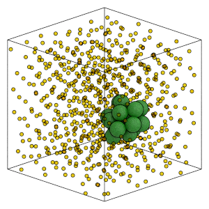
Tracking particles that undergo transitions during simulations is often essential for detailed analysis. Dupin’s logging infrastructure is designed specifically for this purpose. In this example, we will demonstrate how to use the logging functionality to identify and track particles that are undergoing nucleation effectively identifying particles belonging to the critical nucleus. The render function in the next (hidden) cell will render the snapshot at the detected change point using fresnel. You can find the source code for this function on github.

import copy

import freud
import gsd.hoomd
import matplotlib.pyplot as plt
import ruptures as rpt

import dupin as du

ls = 6
FILENAME = "../data/lj-sim.gsd"
steinhardt = freud.order.Steinhardt(l=ls)
logger = du.data.logging.Logger()


# custom generator function
def minkowski_generator(system):
    # compute voronoi neighbors and get nlist
    vor = freud.locality.Voronoi()
    vor.compute(system)
    nlist = vor.nlist
    # compute steinhardt
    steinhardt = freud.order.Steinhardt(l=ls, weighted=True)
    steinhardt.compute(system, neighbors=nlist)
    return dict(M6=steinhardt.particle_order)


pipeline = du.data.base.CustomGenerator(minkowski_generator).pipe(
    du.data.reduce.NthGreatest((-10, -50))
)
signal_aggregator = du.data.aggregate.SignalAggregator(pipeline, logger)
with gsd.hoomd.open(FILENAME, "r") as traj:
    for frame in traj:
        signal_aggregator.accumulate(frame)
lin_regress_cost = du.detect.CostLinearFit()
dynp = rpt.Dynp(custom_cost=lin_regress_cost)
sweep_detector = du.detect.SweepDetector(
    dynp, max_change_points=6, tolerance=0.001
)
change_points = sweep_detector.fit(signal_aggregator.to_dataframe())
change_point_particle_id = logger.frames[change_points[0]]["M6"]["NthGreatest"][
    "10th_least"
]
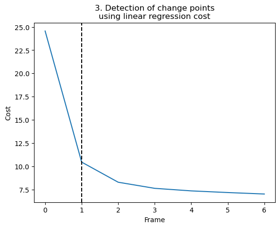
plt.plot(sweep_detector.costs_)
plt.title("3. Detection of change points\nusing linear regression cost")
plt.xlabel("Frame")
plt.ylabel("Cost")
plt.axvline(sweep_detector.opt_n_change_points_, color="k", linestyle="--")
plt.show()
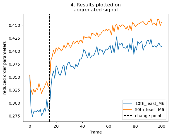
# add change points as vlines
plt.plot(
    signal_aggregator.to_dataframe().to_numpy(),
    label=signal_aggregator.to_dataframe().columns.to_list(),
)
for change_point in change_points:
    plt.axvline(change_point, color="k", linestyle="--", label="change point")
plt.title("4. Results plotted on\naggregated signal")
plt.xlabel("Frame")
plt.ylabel("reduced order parameters")
plt.legend()
plt.show()
with gsd.hoomd.open(FILENAME, "r") as f:
    frame: gsd.hoomd.Frame = f[change_points[0]]
    vor = freud.locality.Voronoi()
    vor.compute((frame.configuration.box, frame.particles.position))
    neighbor_list = vor.nlist
    first_index = neighbor_list.find_first_index(change_point_particle_id)
    num_neighs = neighbor_list.neighbor_counts[change_point_particle_id]
    ids = neighbor_list.point_indices[first_index : first_index + num_neighs]
    ids = ids.tolist()
    ids.append(change_point_particle_id)
    particle_ids = copy.deepcopy(frame.particles.typeid)
    particle_ids[ids] = 1
    newframe = gsd.hoomd.Frame()
    newframe.configuration.box = frame.configuration.box
    newframe.particles.position = frame.particles.position
    newframe.particles.types = frame.particles.types
    newframe.particles.typeid = particle_ids
    img = render(newframe)
    display(img)